Matlab实现季节性时间序列ARIMA模型预测

这段是实现预测的关键代码，需要大家根据个人情况编写剩余代码

参数定义： x为原始序列数据
y为进行周期差分变换后的x
w为差分运算之后的y

话不多说，直接上代码，后面有分段的代码讲解

figure(1);
plot(x,'k-h');
% set(gca,'XTicklabel',{'2005/01','2006/08','2008/04','2009/12','2011/08','2013/04', ...
%     '2014/12','2016/08','2018/04','2019/12','2021/08'});
% xlabel('Time');
% ylabel('Elevation');
% legend('Elevation of Lake Mead : 2005 - 2020');
grid on;
title('Raw data image') %原始数据图像
% subplot(1,2,2)
figure(2);
autocorr(x)
title('Autocorrelation function graph') % 自相关函数图像

%做1阶4步差分
s=12;  %周期s=12
n=18;  %预报数据的个数
m1=length(x); % x的个数
for i=s+1:m1
  	y(i-s)=x(i)-x(i-s);  % 进行周期差分变换
end
w=diff(y,1); % 差分运算，消除趋势性
m2=length(w); w的个数
figure(3);
% subplot(1,2,1)
plot(w);
grid on;
% set(gca,'XTicklabel',{'2005/01','2006/08','2008/04','2009/12','2011/08','2013/04', ...
%     '2014/12','2016/08','2018/04','2019/12','2021/08'});
% xlabel('Time');
% ylabel('Elevation');
% legend('Elevation of Lake Mead Data (2005 - 2020) after The differential');
title('Differential post sequence image') % 差分后序列图像
% subplot(1,2,2)
figure(4);
autocorr(w)
title('Autocorrelation function graph')


% norm test  需要序列服从正态分布
figure(5);
normplot(x);
xlabel('Elevation Data');
ylabel('Posibility');
title('Normal probability graph');
%% select the model

k = 0;
for i = 0 : 3  % 确定模型结构
    for j = 0 : 3
        if i == 0 & j == 0
            continue;
        elseif i == 0
            ToEstMd = arima('MALags',1 : j,'Constant',0);
        elseif j == 0
            ToEstMd = arima('ARLags',1 : i,'Constant',0);
        else
            ToEstMd = arima('ARLags',1 : i,'MALags',1 : j,'Constant',0);
        end
        k = k + 1;R(k) = i;M(k) = j;
        [EstMd,EstParamCov,logL,info] = estimate(ToEstMd,w');
        numParams = sum(any(EstParamCov));
        [aic(k),bic(k)] = aicbic(logL,numParams,m2);
    end
end

fprintf('R,M,AIC,BIC的对应值如下\n%f'); % 根据AIC、BIC准则定阶
check = [R',M',aic',bic']
r = input('输入阶数R = ');m = input('输入阶数M = ');
ToEstMd = arima('ARLags',1 : r,'MALags',1:m,'Constant',0); %指定模型的结构

%% estimate && forecast && results
[EstMd,EstParamCov,logL,info] = estimate(ToEstMd,w');%模型拟合 
w_Forecast = forecast(EstMd,n,'Y0',w');
yhat = y(end) + cumsum(w_Forecast); %一阶差分的还原值
for j = 1:n
    x(m1 + j) = yhat(j) + x(m1+j-s); %x的预测值
end
xhat = x(m1 + 1 : end); % 提取x预测的值

1.首先是将序列变为平稳的

figure(1);
plot(x,'k-h');
% set(gca,'XTicklabel',{'2005/01','2006/08','2008/04','2009/12','2011/08','2013/04', ...
%     '2014/12','2016/08','2018/04','2019/12','2021/08'});
% xlabel('Time');
% ylabel('Elevation');
% legend('Elevation of Lake Mead : 2005 - 2020');
grid on;
title('Raw data image') %原始数据图像
% subplot(1,2,2)
figure(2);
autocorr(x)
title('Autocorrelation function graph') % 自相关函数图像

%做1阶4步差分
s=12;  %周期s=12
n=18;  %预报数据的个数
m1=length(x); % x的个数
for i=s+1:m1
  	y(i-s)=x(i)-x(i-s);  % 进行周期差分变换
end
w=diff(y,1); % 差分运算，消除趋势性
m2=length(w); w的个数
figure(3);
% subplot(1,2,1)
plot(w);
grid on;
% set(gca,'XTicklabel',{'2005/01','2006/08','2008/04','2009/12','2011/08','2013/04', ...
%     '2014/12','2016/08','2018/04','2019/12','2021/08'});
% xlabel('Time');
% ylabel('Elevation');
% legend('Elevation of Lake Mead Data (2005 - 2020) after The differential');
title('Differential post sequence image') % 差分后序列图像
% subplot(1,2,2)
figure(4);
autocorr(w)
title('Autocorrelation function graph')

Figure 1

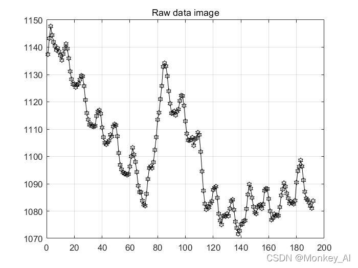
可以看到原序列具有显著的趋势，初步判断为非平稳序列。

再看自相关函数图：

Figure 2

可以看到自相关函数图并未较快的衰减为0，因此该序列并非为平稳的。

1.1 确定季节性周期时间，进行周期性差分变换

确定序列为非平稳之后，在处理平稳性之前先需要做一件事：消除周期性、季节性，这里就用到了差分变换

%做1阶4步差分
s=12;  %周期s=12
n=18;  %预报数据的个数
m1=length(x); % x的个数
for i=s+1:m1
  	y(i-s)=x(i)-x(i-s);  % 进行周期差分变换
end

1.2 如何变为平稳

利用差分运算，对数据进行一阶差分运算，具体用diff函数实现

w=diff(y,1); % 差分运算，消除趋势性
m2=length(w); w的个数
figure(3);
% subplot(1,2,1)
plot(w);
grid on;
% set(gca,'XTicklabel',{'2005/01','2006/08','2008/04','2009/12','2011/08','2013/04', ...
%     '2014/12','2016/08','2018/04','2019/12','2021/08'});
% xlabel('Time');
% ylabel('Elevation');
% legend('Elevation of Lake Mead Data (2005 - 2020) after The differential');
title('Differential post sequence image') % 差分后序列图像
% subplot(1,2,2)
figure(4);
autocorr(w)
title('Autocorrelation function graph')

这里画了两张图，用plot和autocorr函数实现的

Figure 3

Figure 4

可以看到一阶差分之后数据在某个区间内波动，且有界，无明显趋势及周期性特征，判断一阶差分之后序列平稳。

2.正态性检验

% norm test  需要序列服从正态分布
figure(5);
normplot(x);
xlabel('Elevation Data');
ylabel('Posibility');
title('Normal probability graph');

所使用序列应该符合正态分布，可以用matlab的adtest，jbtest或者lillietest等函数进行检验，返回的h值若为0则认为服从正态分布。这里使用normplot函数画正态分布图

Figure 5

可以发现数据基本都位于标线附近，可以认为数据服从正态分布(其实不太严谨但我直接用了hh，差不多就行应该问题不大)

3.模型的遍历选择

%% select the model

k = 0;
for i = 0 : 3  % 确定模型结构
    for j = 0 : 3
        if i == 0 & j == 0
            continue;
        elseif i == 0
            ToEstMd = arima('MALags',1 : j,'Constant',0);
        elseif j == 0
            ToEstMd = arima('ARLags',1 : i,'Constant',0);
        else
            ToEstMd = arima('ARLags',1 : i,'MALags',1 : j,'Constant',0);
        end
        k = k + 1;R(k) = i;M(k) = j;
        [EstMd,EstParamCov,logL,info] = estimate(ToEstMd,w');
        numParams = sum(any(EstParamCov));
        [aic(k),bic(k)] = aicbic(logL,numParams,m2);
    end
end

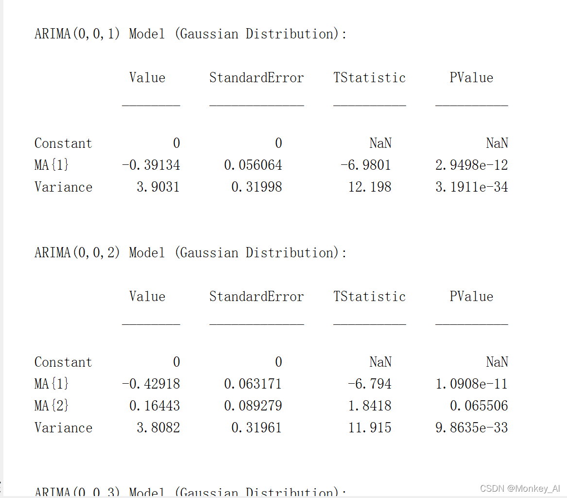
当i == 0，j == 0的时候跳过，其他值的时候进入，(0,1)(0,2)(0,3)(1,0)(1,1)(1,2)......等15(16 - 1)个挨个参数带入arima函数进行计算，同时计算出AIC和BIC值，保存下来。

--------------------------------------------------------------------------------------------------------------------------------

4.定阶

fprintf('R,M,AIC,BIC的对应值如下\n%f'); % 根据AIC、BIC准则定阶
check = [R',M',aic',bic']

在命令行窗口显示R，M，AIC，BIC的值，以列向量的形式表示，然后根据AIC，BIC准则来进行选择模型的阶数。通常，取AIC，BIC最小的值，当AIC与BIC取值冲突时，以AIC为准。

例如第一个751.5379代表的是(0,1) 第四个746.3329代表的是(1,0)

5.代入，出结果

r = input('输入阶数R = ');m = input('输入阶数M = ');
ToEstMd = arima('ARLags',1 : r,'MALags',1:m,'Constant',0); %指定模型的结构

%% estimate && forecast && results
[EstMd,EstParamCov,logL,info] = estimate(ToEstMd,w');%模型拟合 
w_Forecast = forecast(EstMd,n,'Y0',w');
yhat = y(end) + cumsum(w_Forecast); %一阶差分的还原值
for j = 1:n
    x(m1 + j) = yhat(j) + x(m1+j-s); %x的预测值
end
xhat = x(m1 + 1 : end); % 提取x预测的值

分别输入r和m，然后进行计算，estimate函数进行模型拟合，然后forecast函数进行预测。之后进行一阶差分的还原，最后获得x的预测值。

Figure 6

这是预测结果的一些图像

画图的代码放下面了，有兴趣可以看看

%% result plot
clear
clc
D = xlsread('res_forcast_2021-2050_model_2.xlsx');
d_25 = D(49 : 60);
d_30 = D(109 : 120);
d_50 = D(end - 11:end);

figure(6);
fst = plot(d_25);
fst.LineWidth = 3;
fst.Color = 'y';
fst.Marker = '*';
grid on;
hold on;

scd = plot(d_30);
scd.LineWidth = 3;
scd.Color = 'k';
scd.Marker = 'x';

hold on;
thd = plot(d_50);
thd.LineWidth = 3;
thd.Color = 'c'; 
thd.Marker = '^';

legend('In 2025','In 2030', ...
    'In 2050');

xlabel('Month');
ylabel('Elevation');
title('Elevation Of Lake Mead (2025、2030、2050)');

鉴于本人水平有限，有错误的地方还恳请大家指出，批评，共同进步。

原文链接：https://blog.csdn.net/qq_54488033/article/details/122724210