动手学深度学习（三十二）——全连接卷积神经网络FCN

1. 什么是全卷积神经网络（Fully Convolutional Networks）

在图像分类任务中我们通常使用CNN+全连接层，将卷积层产生的特征图(feature map)映射成一个固定长度的特征向量。以AlexNet为例，由于图像分类最后期望得到整个输入图像的一个数值描述（概率），比如AlexNet的ImageNet模型输出一个1000维的向量表示输入图像属于每一类的概率(softmax归一化)。

例如：下面这张图中表示，输入图片，使用AlexNet分析，得到一个长度为1*1000的向量，然后根据这个向量判断这张图的类别是猫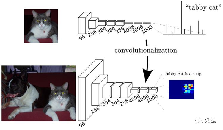

传统的CNN有问题：

1. 存储开销大
   • 滑动窗口较大，每个窗口都需要存储空间来保存特征和判别类别
   • 使用全连接结构，最后几层将近指数级存储递增
2. 计算效率低。存在大量重复计算
3. 滑动窗口是独立的，末端使用全连接层只是为了局部特征。

针对这些问题，如果将模型中的全连接层全部换为卷积层可以在一定程度上解决问题，我们将这个全部由卷积层构成的网络称为全卷积神经网络FCN。

2. FCN是语义分割的奠基性工作

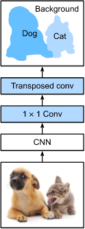
使用转置卷积替换CNN最后的全连接层，从而实现对每个像素的预测，达到语义分割的目的

3. 使用FCN进行语义分割

%matplotlib inline
import torch 
import torchvision
from torch import nn 
from torch.nn import functional as F 
from d2l import torch as d2l 
import os

3.1 模型构建

# 使用在ImageNet数据集上预训练的ResNet-18进行图像特征的提取，并将网络实例记为pretrained_net
# 注意ResNet-18的最后几层是全局平均池化层和全连接层，在FCN中不需要
pretrained_net = torchvision.models.resnet18(pretrained=True)
list(pretrained_net.children())[-3:]

[Sequential(
   (0): BasicBlock(
     (conv1): Conv2d(256, 512, kernel_size=(3, 3), stride=(2, 2), padding=(1, 1), bias=False)
     (bn1): BatchNorm2d(512, eps=1e-05, momentum=0.1, affine=True, track_running_stats=True)
     (relu): ReLU(inplace=True)
     (conv2): Conv2d(512, 512, kernel_size=(3, 3), stride=(1, 1), padding=(1, 1), bias=False)
     (bn2): BatchNorm2d(512, eps=1e-05, momentum=0.1, affine=True, track_running_stats=True)
     (downsample): Sequential(
       (0): Conv2d(256, 512, kernel_size=(1, 1), stride=(2, 2), bias=False)
       (1): BatchNorm2d(512, eps=1e-05, momentum=0.1, affine=True, track_running_stats=True)
     )
   )
   (1): BasicBlock(
     (conv1): Conv2d(512, 512, kernel_size=(3, 3), stride=(1, 1), padding=(1, 1), bias=False)
     (bn1): BatchNorm2d(512, eps=1e-05, momentum=0.1, affine=True, track_running_stats=True)
     (relu): ReLU(inplace=True)
     (conv2): Conv2d(512, 512, kernel_size=(3, 3), stride=(1, 1), padding=(1, 1), bias=False)
     (bn2): BatchNorm2d(512, eps=1e-05, momentum=0.1, affine=True, track_running_stats=True)
   )
 ),
 AdaptiveAvgPool2d(output_size=(1, 1)),
 Linear(in_features=512, out_features=1000, bias=True)]

# 根据pretrained net创建一个新的网络实例，去除FCN不需要的部分
net = nn.Sequential(*list(pretrained_net.children())[:-2])

# 给定高宽为(320*480)的输入，net的前向网络将输入的高宽缩小到原来的1/32,即(10，15)
X = torch.rand(size=(1,3,320,480))
net(X).shape

torch.Size([1, 512, 10, 15])

# 使用1*1的卷积层将输出通道数转换为Pascal VO2012数据集的类别数（21类）.
# 这里的输出通道数选择21的原因是为了减少后面transpose层的计算量(减少到最小)
num_classes =21
net.add_module('final_conv',nn.Conv2d(512,num_classes,kernel_size=1))

使用转置卷即将要素图的高度和宽度增加32倍，恢复到输入图像的高和宽

由于$(320-64+16\times 2+32)/32=10$且$(480-64+16\times 2+32)/32=15$，我们构造一个步幅为$32$的转置卷积层，并将卷积核的高和宽设为$64$，填充为$16$。
我们可以看到如果步幅为$s$，填充为$s/2$（假设$s/2$是整数）且卷积核的高和宽为$2s$，转置卷积核会将输入的高和宽分别放大$s$倍。

net.add_module('transpose_conv',nn.ConvTranspose2d(num_classes,num_classes,kernel_size=64,padding=16,stride=32))

3.2 初始化转置卷积层

在图像处理中，我们有时需要将图像放大，即上采样(upsampling)。

双线性插值（bilinear interpolation）是常用的上采样方法之一，它也经常用于初始化转置卷积层。为了解释双线性插值，假设给定输入图像，我们想要计算上采样输出图像上的每个像素。

• 首先，将输出图像的坐标$(x,y)$映射到输入图像的坐标$(x^{\prime },y^{\prime })$上。例如，根据输入与输出的尺寸之比来映射。请注意，映射后的$x\prime$和$y\prime$是实数。
• 然后，在输入图像上找到离坐标$(x^{\prime },y^{\prime })$最近的4个像素。
• 最后，输出图像在坐标$(x,y)$上的像素依据输入图像上这4个像素及其与$(x^{\prime },y^{\prime })$的相对距离来计算。

双线性插值的上采样可以通过转置卷积层实现，内核由以下bilinear_kernel函数构造。
限于篇幅，我们只给出bilinear_kernel函数的实现，不讨论算法的原理

def bilinear_kernel(in_channels, out_channels, kernel_size):
    factor = (kernel_size + 1) // 2
    if kernel_size % 2 == 1:
        center = factor - 1
    else:
        center = factor - 0.5
    og = (torch.arange(kernel_size).reshape(-1, 1),
          torch.arange(kernel_size).reshape(1, -1))
    filt = (1 - torch.abs(og[0] - center) / factor) * \
           (1 - torch.abs(og[1] - center) / factor)
    weight = torch.zeros(
        (in_channels, out_channels, kernel_size, kernel_size))
    weight[range(in_channels), range(out_channels), :, :] = filt
    return weight

# 这里使用转置层实现双线性差值，构建一个输入高宽放大两倍的转置卷积层，并将卷积核使用`bilinear_kernel`函数构建
conv_trans = nn.ConvTranspose2d(3,3,kernel_size=4,padding=1,stride=2,bias=False)
conv_trans.weight.data.copy_(bilinear_kernel(3,3,4))

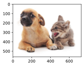
# 读取图像X，将上采样的结果记为Y,为了输出打印图片需要调整维度
img = torchvision.transforms.ToTensor()(d2l.Image.open('./course_file/pytorch/img/catdog.jpg'))
X = img.unsqueeze(0)
Y = conv_trans(X)
out_img = Y[0].permute(1, 2, 0).detach()
d2l.set_figsize()
print('input image shape:', img.permute(1, 2, 0).shape)
d2l.plt.imshow(img.permute(1, 2, 0))

input image shape: torch.Size([561, 728, 3])

print('output image shape:', out_img.shape)
d2l.plt.imshow(out_img);

可以看到，转置卷积层将图像的高和宽分别放大了2倍。除了坐标刻度不同，双线性插值放大的图像和原图看上去没什么两样。所以我们在全卷积网络中，[用双线性插值的上采样初始化转置卷积层。对于$1\times 1$卷积层，我们使用Xavier初始化参数。]

W = bilinear_kernel(num_classes, num_classes, 64)
net.transpose_conv.weight.data.copy_(W);

3.3 读取数据集

我们用https://blog.csdn.net/jerry_liufeng/article/details/120820270 介绍的方法数据集。
指定随机裁剪的输出图像的形状为$320\times 480$：高和宽都可以被$32$整除。

#@save
def read_voc_images(voc_dir, is_train=True):
    """读取所有VOC图像并标注。"""
    txt_fname = os.path.join(voc_dir, 'ImageSets', 'Segmentation',
                             'train.txt' if is_train else 'val.txt')
    mode = torchvision.io.image.ImageReadMode.RGB
    with open(txt_fname, 'r') as f:
        images = f.read().split()
    features, labels = [], []
    for i, fname in enumerate(images):
        features.append(
            torchvision.io.read_image(
                os.path.join(voc_dir, 'JPEGImages', f'{fname}.jpg')))
        # 对于语义分割，要求对每一个像素进行分类，所以label保存为一个没有经过压缩的.png文件是比较合适的
        labels.append(
            torchvision.io.read_image(
                os.path.join(voc_dir, 'SegmentationClass', f'{fname}.png'),
                mode))
    return features, labels

#@save
VOC_COLORMAP = [[0, 0, 0], [128, 0, 0], [0, 128, 0], [128, 128, 0],
                [0, 0, 128], [128, 0, 128], [0, 128, 128], [128, 128, 128],
                [64, 0, 0], [192, 0, 0], [64, 128, 0], [192, 128, 0],
                [64, 0, 128], [192, 0, 128], [64, 128, 128], [192, 128, 128],
                [0, 64, 0], [128, 64, 0], [0, 192, 0], [128, 192, 0],
                [0, 64, 128]]

#@save
VOC_CLASSES = [
    'background', 'aeroplane', 'bicycle', 'bird', 'boat', 'bottle', 'bus',
    'car', 'cat', 'chair', 'cow', 'diningtable', 'dog', 'horse', 'motorbike',
    'person', 'potted plant', 'sheep', 'sofa', 'train', 'tv/monitor']

"""
定义函数将RGB颜色列别和类别索引进行映射
"""

#@save
def voc_colormap2label():
    """构建从RGB到VOC类别索引的映射。"""
    colormap2label = torch.zeros(256**3, dtype=torch.long)
    for i, colormap in enumerate(VOC_COLORMAP):
        colormap2label[(colormap[0] * 256 + colormap[1]) * 256 +
                       colormap[2]] = i
    return colormap2label

#@save
def voc_label_indices(colormap, colormap2label):
    """将VOC标签中的RGB值映射到它们的类别索引。"""
    colormap = colormap.permute(1, 2, 0).numpy().astype('int32')
    idx = ((colormap[:, :, 0] * 256 + colormap[:, :, 1]) * 256 +
           colormap[:, :, 2])
    return colormap2label[idx]

#@save
def voc_rand_crop(feature, label, height, width):
    """随机裁剪特征和标签图像。"""
    rect = torchvision.transforms.RandomCrop.get_params(
        feature, (height, width))
    feature = torchvision.transforms.functional.crop(feature, *rect)
    label = torchvision.transforms.functional.crop(label, *rect)
    return feature, label

#@save
class VOCSegDataset(torch.utils.data.Dataset):
    """一个用于加载VOC数据集的自定义数据集。"""
    def __init__(self, is_train, crop_size, voc_dir):
        self.transform = torchvision.transforms.Normalize(
            mean=[0.485, 0.456, 0.406], std=[0.229, 0.224, 0.225])
        self.crop_size = crop_size
        features, labels = read_voc_images(voc_dir, is_train=is_train)
        self.features = [
            self.normalize_image(feature)
            for feature in self.filter(features)]
        self.labels = self.filter(labels)
        self.colormap2label = voc_colormap2label()
        print('read ' + str(len(self.features)) + ' examples')

    def normalize_image(self, img):
        return self.transform(img.float())

    def filter(self, imgs):
        return [
            img for img in imgs if (img.shape[1] >= self.crop_size[0] and
                                    img.shape[2] >= self.crop_size[1])]

    def __getitem__(self, idx):
        feature, label = voc_rand_crop(self.features[idx], self.labels[idx],
                                       *self.crop_size)
        return (feature, voc_label_indices(label, self.colormap2label))

    def __len__(self):
        return len(self.features)

#@save
def load_data_voc(batch_size, crop_size):
    """
    加载VOC语义分割数据集。
    """
    # voc_dir = d2l.download_extract('voc2012',
    #                                os.path.join('VOCdevkit', 'VOC2012'))
    voc_dir = os.path.join("../data/VOCdevkit/VOC2012/")
    num_workers = d2l.get_dataloader_workers()
    train_iter = torch.utils.data.DataLoader(
        VOCSegDataset(True, crop_size, voc_dir), batch_size, shuffle=True,
        drop_last=True, num_workers=num_workers)
    test_iter = torch.utils.data.DataLoader(
        VOCSegDataset(False, crop_size, voc_dir), batch_size, drop_last=True,
        num_workers=num_workers)
    return train_iter, test_iter

batch_size, crop_size = 24, (320, 480)
train_iter, test_iter = load_data_voc(batch_size, crop_size)

read 1114 examples
read 1078 examples

3.4 训练

def loss(inputs, targets):
    return F.cross_entropy(inputs, targets, reduction='none').mean(1).mean(1)

num_epochs, lr, wd, devices = 5, 0.001, 1e-3, d2l.try_all_gpus()
trainer = torch.optim.SGD(net.parameters(), lr=lr, weight_decay=wd)

# 多GPU训练和评估
def train_batch(net, X, y, loss, trainer, devices):
    if isinstance(X, list):
        # 微调BERT中所需（稍后讨论）
        X = [x.to(devices[0]) for x in X]
    else:
        X = X.to(devices[0])
    y = y.to(devices[0])
    net.train()
    trainer.zero_grad()
    pred = net(X)
    l = loss(pred, y)
    l.sum().backward()
    trainer.step()
    train_loss_sum = l.sum()
    train_acc_sum = d2l.accuracy(pred, y)
    return train_loss_sum, train_acc_sum


def train(net, train_iter, test_iter, loss, trainer, num_epochs,
               devices=d2l.try_all_gpus()):
    timer, num_batches = d2l.Timer(), len(train_iter)
    animator = d2l.Animator(xlabel='epoch', xlim=[1, num_epochs], ylim=[0, 1],
                            legend=['train loss', 'train acc', 'test acc'])
    net = nn.DataParallel(net, device_ids=devices).to(devices[0]) # 多GPU运行
    for epoch in range(num_epochs):
        # 4个维度：储存训练损失，训练准确度，实例数，特点数
        metric = d2l.Accumulator(4)
        for i, (features, labels) in enumerate(train_iter):
            timer.start()
            l, acc = train_batch(net, features, labels, loss, trainer,
                                      devices)
            metric.add(l, acc, labels.shape[0], labels.numel())
            timer.stop()
            if (i + 1) % (num_batches // 5) == 0 or i == num_batches - 1:
                animator.add(
                    epoch + (i + 1) / num_batches,
                    (metric[0] / metric[2], metric[1] / metric[3], None))
            print(metric[0]/metric[2])
        test_acc = d2l.evaluate_accuracy_gpu(net, test_iter)
        animator.add(epoch + 1, (None, None, test_acc))
    print(f'loss {metric[0] / metric[2]:.3f}, train acc '
          f'{metric[1] / metric[3]:.3f}, test acc {test_acc:.3f}')
    print(f'{metric[2] * num_epochs / timer.sum():.1f} examples/sec on '
          f'{str(devices)}')

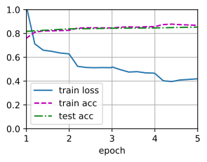
train(net, train_iter, test_iter, loss, trainer, num_epochs, devices)

loss 0.420, train acc 0.869, test acc 0.854
0.8 examples/sec on [device(type='cuda', index=0)]

3.5 预测

预测时需要将输入图像在各个通道做标准化，并转换成卷积神经网络的四维输入格式

def predict(img):
    X = test_iter.dataset.normalize_image(img).unsqueeze(0)
    pred = net(X.to(devices[0])).argmax(dim=1)
    return pred.reshape(pred.shape[1],pred.shape[2])

为了[可视化预测的类别]给每个像素，我们将预测类别映射回它们在数据集中的标注颜色。

def label2image(pred):
    colormap = torch.tensor(d2l.VOC_COLORMAP, device=devices[0])
    X = pred.long()
    return colormap[X, :]

测试数据集中的图像大小和形状各异。

由于模型使用了步幅为32的转置卷积层，因此当输入图像的高或宽无法被32整除时，转置卷积层输出的高或宽会与输入图像的尺寸有偏差。

为了解决这个问题，我们可以在图像中截取多块高和宽为32的整数倍的矩形区域，并分别对这些区域中的像素做前向计算。请注意，这些区域的并集需要完整覆盖输入图像。当一个像素被多个区域所覆盖时，它在不同区域前向计算中转置卷积层输出的平均值可以作为softmax运算的输入，从而预测类别。

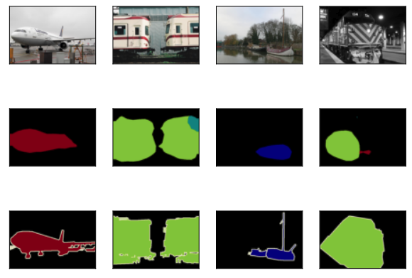
为简单起见，我们只读取几张较大的测试图像，并从图像的左上角开始截取形状为$320\times 480$的区域用于预测。
对于这些测试图像，我们逐一打印它们截取的区域，再打印预测结果，最后打印标注的类别。

voc_dir = os.path.join("../data/VOCdevkit/VOC2012/")
test_images, test_labels = d2l.read_voc_images(voc_dir, False)
n, imgs = 4, []
for i in range(n):
    crop_rect = (0, 0, 320, 480)
    X = torchvision.transforms.functional.crop(test_images[i], *crop_rect)
    pred = label2image(predict(X))
    imgs += [
        X.permute(1, 2, 0),
        pred.cpu(),
        torchvision.transforms.functional.crop(test_labels[i],
                                               *crop_rect).permute(1, 2, 0)]
d2l.show_images(imgs[::3] + imgs[1::3] + imgs[2::3], 3, n, scale=2);

4. 总结

1. 全卷积网络先使用卷积神经网络抽取图像特征，然后通过1*1的卷积层将通道数转换为类别个数，最后通过转置卷积层将特征图的高和宽度变换为输入图像的尺寸。
2. 在全卷积网络中，我们可以将转置卷积层初始化为双线性插值的上采样。
3. 转置卷积层参数的计算参考https://blog.csdn.net/jerry_liufeng/article/details/120816608?spm=1001.2014.3001.5501
4. 最后的语义分析的结果其实并不是非常好，这和我的迭代次数和网络层构建有关
5. 由于输入数据的大小为360*480,每一个batch有36张图，对GPU显存的要求是比较大的，所以训练的时候可能需要调整相应的大小（我仅仅调整了batch的大小为24）。但是训练的效率还是非常低下