基础
一.读取数据
read.csv()
readxl::read.xlsx()
使用read.xlsx时提示:Error: could not find function "read.xlsx"; could not find function "read.xlsx"
原因在于要安装rJava这个包。而安装这个包,需要先在电脑里安装Java程序才行。干脆转换为csv文件导入。
在我打开练习题时出现无法打开文件cannot open file '21-50数据.csv': No such file or directory,是因为我的R软件工作目录路径与文件的保存目录路径不一致导致的
解决方法:
1.读取时写上文件的全路径
df2<-read.csv("C:\\Users\\lenovo\\Desktop\\21-50数据.csv")#windows系统一定要用\\
2、将文件放到当前R的工作目录
首先要获取当前R的工作目录,使用 getwd()
3、将文件所在目录设置为R的工作目录
重新设置R的工作目录,使用 setwd()
二、计算
1.将salary数据转换为最大值与最小值的平均值
df2 = df2 %>%
separate(salary, into = c("low", "high"), sep = "-") %>% # sep="-" 也可以省略#分成高低两组
mutate(salary = (parse_number(low) + parse_number(high)) * 1000 / 2) %>%# parse_number()指提取变量中的数字部分
select(-c(low, high))
2.(分组汇总):根据学历分组,并计算平均薪资
df2<-df2%>%
group_by(education)%>%
summarise(salary_avg=mean(salary))
3.(时间转换):将 createTime 列转换为 “月-日”
library(lubridate)
df2 %>%
mutate(createTime = str_c(month(createTime), "-", day(createTime)))#str_c合并字符
4.查看数据结构信息
df %>% glimpse() # 或者用 str()
object.size(df) # 查看对象占用内存
5.新增一列将 salary 离散化为三水平值
1.case_when函数
df = df %>%
mutate(class = case_when(
salary >= 0 & salary < 5000 ~ " 低",
salary >= 5000 & salary < 20000 ~ " 中",
TRUE ~ " 高")) # TRUE 效果是其它
2.cut函数:要将连续型变量变成离散型因子,需要对连续型变量进行切割,每个区间可成为一个因子。可以用cut函数完成连续型变量的切割工作。
df %>%
mutate(class = cut(salary,
breaks = c(0,5000,20000,Inf),
labels = c(" 低", " 中", " 高"),
right = FALSE))#逻辑值,默认为TRUE(左开右闭);FALSE(左闭右开)
6.按 salary 列对数据降序排列
df2<-df2%>%
arrange(desc(salary)
arrange(-salary)
7.提取第 33 行数据
df %>% slice(33)或
df2[33,]
8.计算 salary 列的中位数
df2%>%
summarise(salary_median=median(salary))或
median(df2$salary)
9.绘制 salary 的频率分布直方图
library(ggplot2)
ggplot(df2,aes(x=salary))+
geom_histogram(bins = 10)
这里会出现问题:因为salary不是连续型变量
StatBin requires a continuous x variable: the x variable is discrete.Perhaps you want stat="count"?
使用
stat_count(width = 0.5)而不是geom_bar()或geom_histogram(binwidth = 0.5)将解决它。
10.绘制 salary 的频率密度曲线图
df %>%
ggplot(aes(x = salary)) +
geom_density()
画图时出现报错:
Warning message:
Removed 135 rows containing non-finite values (stat_bin).
11.删除最后一列 class
df %>% select(-class)或者
同#6的补充,给class列赋空值即删去,如下
df %>%mutate(class = NULL)或者
df %>% select(-last_col()) # 同 last_col(0)
12.将 df 的第 1 列与第 2 列合并为新的一列
df %>%
unite("newcol", 1:2, sep = " ")
unite函数用法
unite(data,"newcolname",colname1,colname2,sep=":",remove=FALSE)
remove=TRUE移除原本两行cbind: 根据列进行合并,即叠加所有列,m列的矩阵与n列的矩阵cbind()最后变成m+n列,合并前提:cbind(a, c)中矩阵a、c的行数必需相符。感觉cbind是合并数据框?
13.将 education 列与第 salary 列合并为新的一列
df2%>%unite("newcol2",c(education, salary),sep="",remove=TRUE)
14.计算 salary 最大值与最小值之差
max(df2$salary)-mean(df2$salary)或者
df %>% summarise(range = max(salary) - min(salary))
15.将第一行与最后一行拼接
df %>% slice(1, n())或者
bind_rows(df[1,], df[nrow(df),])
# 第一行df[1,]
# 最后一行df[nrow(df),]
综上在一个数据文件内合并列用unite
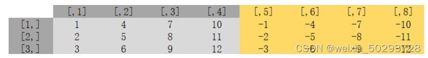
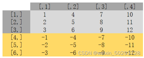
cbind和rbind是针对向量,数据框进行操作的。bind_cols、cbind按行合并,bind_row、rbind按列合并,每个对象必须有相同行数或列数
cbind合并结果
rbind合并结果
16.将第 8 行添加到末尾
df %>% bind_rows(slice(., 8))或
bind_rows(df, df[8,])
#将第八行合并至末尾,同#38
%>%
tail()
# 显示末尾行
17.将createTime列设置为行索引
distinct()函数是从数据框中筛选出唯一/不同的行
df%>%
distinct(createtime,.keep_all=TRUE)%>% #将createtime挑选出来,If TRUE, keep all variables in .data
column_to_rownames("createtime")%>%#library(tidyverse),将特定列转换成行名,row_to_colnames将特定行转换为列
head()
18.生成一个和df长度相同的随机数数据框
df1=tibble(rnums=sample.int(10,nrow(df),replace=TRUE))
# 创建这样的一个tibble数据框,将随机数赋值给rnums,要求为:数据为10以内正整数,数量同df,可以重复
19.将上面生成的数据框与df按列合并
df = bind_cols(df, df1)
20.生成新列new为salary列减去随机数列
df=df%>%
mutate(new=salary-rnums)
21.检查数据众是否含有任何缺失值
anyNA(df)
22.将rnums列的类型转换为浮点数
df%>%
mutate(rnums=as.double(rnums))
rnums为int型(整数),使用as.double进行转换,其他形式也类比
23.计算salary列大于10000的次数
df%>%
summarise(n=sum(salary>10000))或者
df%>%count(salary>10000)
24.查看每种学历出现的次数
df%>%
summarise(n=education)或者
df%>%count(education)
25.查看education里有几种学历
df%>%
distinct(education)
26.提取salary与new列之和大于6000的最后三行
df%>%
filter(salary+new>6000)%>%
slice_head(n=3)
slice包
slice_head() and slice_tail() select the first or last rows.
slice_sample() randomly selects rows.
slice_min() and slice_max() select rows with highest or lowest values of a variable.