k-NN算法，构建模型只需要保存训练数据集，对新数据点做出预测，算法会在数据集中找到最近的数据点（最近邻）。

k近邻分类：KNeighborsClassifier

1邻居直接取邻居，多邻居取出出现次数较多的。
可视化：mglearn.plots.plot_knn_classification(n_neighbors=3)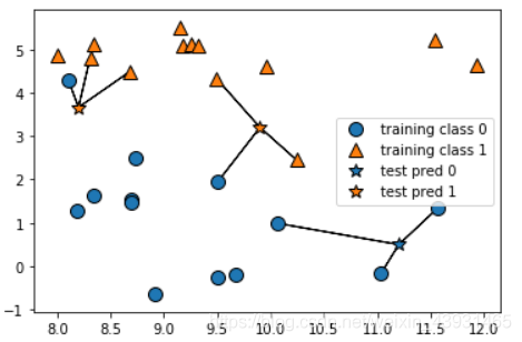

在forge数据集上的应用

from sklearn.model_selection import train_test_split

# 生成数据集
X, y = mglearn.datasets.make_forge() # 输入，目标
X_train, X_test, y_train, y_test = train_test_split(X, y, random_state=0)

# 构建模型
from sklearn.neighbors import KNeighborsClassifier
clf = KNeighborsClassifier(n_neighbors=3)
clf.fit(X_train, y_train) # 利用训练集对分类器进行拟合

# 评估模型
print(clf.predict(X_test))
print("Test accuracy:{:.2f}".format(clf.score(X_test, y_test))) # 0.86

分析算法

对于二维数据集，绘制可视化图表中，可以查看决策边界（边界这边是一目标类，另外一边是另一目标类）

# 绘制多个画布
fig, axes = plt.subplots(1, 3, figsize=(10, 3))

for n, ax in zip([1, 3, 9], axes):
    clf = KNeighborsClassifier(n_neighbors=n).fit(X, y)
    
    # 绘制分界线
    mglearn.plots.plot_2d_separator(clf, X, fill=True, eps=0.5, ax=ax, alpha=.4)
    
    mglearn.discrete_scatter(X[:, 0], X[:, 1], y, ax=ax)
    ax.set_title("{} neighbor(s)".format(n))
    ax.set_xlabel("feature 0")
    ax.set_ylabel("feature 1")
axes[0].legend(['Class 0', 'Class 1'], loc=3)

在matplotlib下，一个Figure对象可以包含多个子图（Axes）
subplot()函数快速绘制，subplot(numRows, numCols, plotNum)参数为（行号，列号，对象坐在区域）。figsize参数指定以英寸为单位的宽高。facecolor背景色，edgecolor边框色。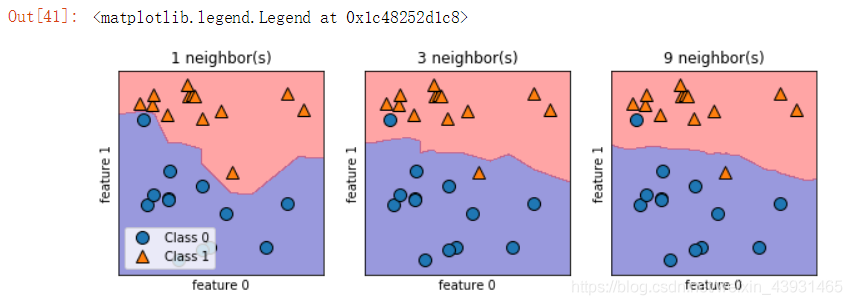

k越大，邻居个数越多，决策边界越平滑，模型越简单（模型复杂度越低）。

在cancer数据集上的应用

from sklearn.datasets import load_breast_cancer

cancer = load_breast_cancer() # Bunch对象
x_train, x_test, y_train, y_test = train_test_split(
    cancer.data, cancer.target, stratify=cancer.target, random_state=66)

training_accuracy = []
test_accuracy = []
neighbors_settings = range(1, 11)

for n in neighbors_settings:
    clf = KNeighborsClassifier(n_neighbors=n).fit(x_train, y_train)
    
    # 训练集精度
    training_accuracy.append(clf.score(x_train, y_train))
    
    # 泛化（测试集）精度
    test_accuracy.append(clf.score(x_test, y_test))

plt.plot(neighbors_settings, training_accuracy, label='training_accuracy')
plt.plot(neighbors_settings, test_accuracy, label='test_accuracy')
plt.legend()

score函数提供了一个缺省的评估法则来解决问题，用训练好的模型在测试集上进行评分（0~1）。
stratify参数作用是：保持测试集与整个数据集里target的数据分类比例一致。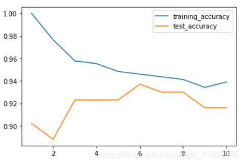

模型复杂度：高->低
过拟合->最佳模型（约88%精度）->欠拟合

k近邻回归：KNeighborsRegressor

多个近邻是，预测结果为邻居的平均值。
可视化：mglearn.plots.plot_knn_regression(n_neighbors=3)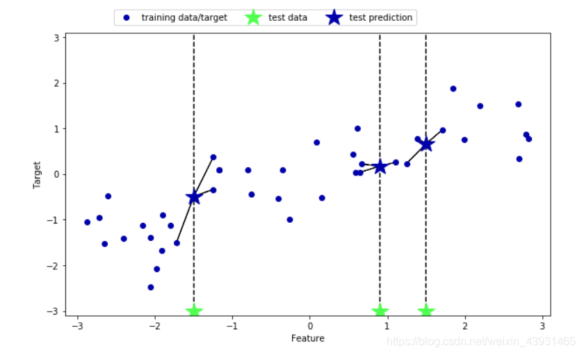

在wave数据集上的应用

from sklearn.neighbors import KNeighborsRegressor
from sklearn.model_selection import train_test_split

x, y = mglearn.datasets.make_wave(n_samples=40)
x_train, x_test, y_train, y_test = train_test_split(x, y, random_state=0)

reg = KNeighborsRegressor(n_neighbors=3)

reg.fit(x_train, y_train)

print(reg.score(x_test, y_test))
print(reg.predict(x_test))
print(y_test) # 0.834...

score方法评估模型，在回归问题，返回R^2分数/决策系数（0-1），是回归模型的优度度量。=1完美预测，=0对应常数模型（总是预测训练集响应的平均值）

分析算法

# 创建画布
fig, axes = plt.subplots(1, 3, figsize=(15, 4))

# 创建1000个均匀分布的数据点
line = np.linspace(-3, 3, 1000).reshape(-1, 1)

for n, ax in zip([1, 3, 7], axes):
    reg = KNeighborsRegressor(n_neighbors=n).fit(x_train, y_train)
    
    ax.plot(x_train, y_train)
    ax.plot(line, reg.predict(line))
    ax.plot(x_train, y_train, '^', c=mglearn.cm2(0), markersize=8) # 指定颜色，标记大小
    ax.plot(x_test, y_test, 'o', c=mglearn.cm2(1),markersize=8)
    ax.set_title('{} nerghbors\n train score:{:.2f} test score:{:.2f}'.format(n,reg.score(x_train,y_train),reg.score(x_test,y_test)))
    ax.set_xlabel('Feature')
    ax.set_ylabel('Target')
axes[0].legend(['Model prediction','Training data/target','Test data/target'],loc='best')

linspace(x1,x2,N)函数，其中x1、x2、N分别为起始值、中止值、元素个数。若缺省N，默认点数为100
reshape(行，列)函数可以根据指定的数值将数据转换为特定的行数和列数。reshape(-1,1)之后，数据集变成了一列。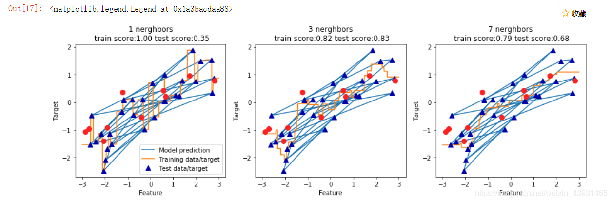

更多邻居后，预测结果更加平滑，但是对训练数据拟合不足。

参数

KNeighbors分类器有2个重要参数：邻居个数、数据点之间距离的度量方法。
距离默认使用欧氏距离。

优缺点

优：模型容易理解；构建模型速度快
缺：预测速度慢且不能处理具有很多特征的数据集