嗨，大家好， (Hi everyone,)

In this article, I will attempt to explain how we can find a confidence interval by using Bootstrap Method. Statistics and Python knowledge are needed for better understanding.

在本文中，我将尝试解释如何使用Bootstrap方法找到置信区间。 需要统计信息和Python知识才能更好地理解。

Before diving into the method, let’s remember some statistical concepts.

在深入探讨该方法之前，让我们记住一些统计概念。

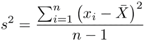
Variance:It is obtained by the sum of squared distances between a data point and the mean for each data point divided by the number of data points.

方差：通过将数据点与每个数据点的平均值之间的平方距离之和除以数据点数而获得。

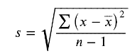
Standard Deviation: It is a measurement that shows us how our data points spread out from the mean. It is obtained by taking the square root of the variance

标准差：这是一项度量，它向我们显示了数据点如何从均值散布。 通过求方差的平方根获得

Cumulative Distribution Function: It can be used on any kind of variable X(discrete, continuous, etc.). It shows us the probability distribution of a variable. Therefore allowing us to interpret the probability of a value less than or equal to x from a given probability distribution

累积分布函数 ：可用于任何类型的变量X(离散，连续等)。 它向我们展示了变量的概率分布。 因此，允许我们根据给定的概率分布来解释小于或等于x的值的概率

Empirical Cumulative Distribution Function: Also known as Empirical Distribution Function. The only difference between CDF and ECDF is, while the former shows us the hypothetical distribution of any given population, the latter is based on our observed data.

经验累积分布函数：也称为经验分布函数。 CDF和ECDF之间的唯一区别是，前者向我们展示了任何给定总体的假设分布，而后者则基于我们的观察数据。

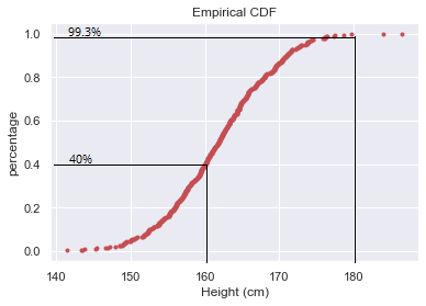
For example, how can we interpret the ECDF of the data shown on the chart above? We can say that 40% of heights are less than or equal to 160cm. Likewise, the percentage of people with heights of less than or equal to 180 cm is 99.3%

例如，我们如何解释上表所示数据的ECDF？ 可以说40％的高度小于或等于160cm。 同样，身高小于或等于180厘米的人的百分比是99.3％

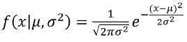
Probability Density Function: It shows us the distribution of continuous variables. The area under the curve gives us the probability so that the area must always be equal to 1

概率密度函数：它向我们展示了连续变量的分布。 曲线下的面积为我们提供了概率，因此该面积必须始终等于1

Normal Distribution: Also known as Gaussian Distribution. It is the most important probability distribution function in statistics which is bell-shaped and symmetric.

正态分布：也称为高斯分布 。 它是钟形和对称的统计中最重要的概率分布函数。

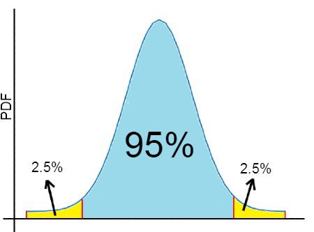
Confidence Interval:It is the range in which the values likely to exist in the population. It is estimated from the original sample and usually defined as 95% confidence but it may differ. You can consider the figure below which indicates a 95% confidence interval. The lower and upper limits of confidence interval defined by the values corresponding to the first and last 2.5th percentiles.

置信区间：这是总体中可能存在的值的范围。 它是根据原始样本估算的，通常定义为95％置信度，但可能有所不同。 您可以考虑下图，它表示置信区间为95％。 置信区间的上限和下限由与第一个和最后一个第2.5个百分点相对应的值定义。

什么是Bootstrap方法？ (What is Bootstrap Method?)

Bootstrap Method is a resampling method that is commonly used in Data Science. It has been introduced by Bradley Efron in 1979. Mainly, it consists of the resampling our original sample with replacement (Bootstrap Sample) and generating Bootstrap replicates by using Summary Statistics.

Bootstrap方法是数据科学中常用的重采样方法。 它由布拉德利·埃夫隆(Bradley Efron)在1979年推出。主要包括重新采样原始样本并进行替换( Bootstrap Sample )，并使用Summary Statistics生成Bootstrap副本 。

人们身高的置信区间 (Confidence Interval of people heights)

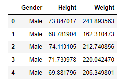
In this article, we are going to work with one of the datasets in Kaggle. It is Weight-Height data sets. It contains height (in inches) and weight (in pounds) information of 10.000 people separated by gender.

在本文中，我们将使用Kaggle中的一个数据集。 它是重量-高度数据集。 它包含按性别分隔的10.000人的身高(英寸)和体重(磅)信息。

If you would like to see the whole code, you can find the IPython notebook via thislink.

如果您想查看整个代码，可以通过此 链接 找到 IPython笔记本。

We are going to use only heights of 500 randomly selected people and compute a 95% confidence interval by using Bootstrap Method

我们将仅使用500个随机选择的人员的身高，并使用Bootstrap方法计算95％的置信区间

Let’s start with importing the libraries that we will need.

让我们从导入所需的库开始。

The first five rows of the DataFrame like following

DataFrame的前五行如下所示

Apparently, heights are in inches, let’s convert heights from inches to centimeters and store in a new column Height(cm).

显然，高度以英寸为单位 ，让我们将高度从英寸转换为厘米，并存储在新列Height(cm)中 。

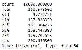
As we can see above, the maximum and minimum height in the data set are 137.8 cm and 200.6 cm respectively.

从上面我们可以看到，数据集中的最大高度和最小高度分别为137.8 cm和200.6 cm。

We can use pandas.DataFrame’s sample method to select 500 randomly selected heights. After that, we will print the summary statistics.

我们可以使用pandas.DataFrame的样本方法来选择500个随机选择的高度。 之后，我们将打印摘要统计信息。

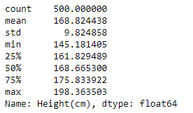
According to the output, our sample has 145 cm as minimum height and 198 cm as the maximum height.

根据输出，我们的样本的最小高度为145厘米，最大高度为198厘米。

Let’s look at how ECDF and PDF look like?

让我们看看ECDF和PDF的外观如何？

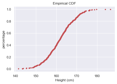
Empirical CDF demonstrates that 50% of people in our sample have 162 cm or less height.

经验CDF证明样本中50％的人身高在162厘米以下。

What about PDF?

那PDF呢？

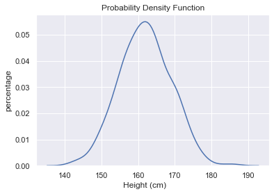
PDF shows us the heights’ distribution is too close to the normal distribution. Do not forget that the area under the curvegives us the probability.

PDF显示高度的分布与正态分布过于接近。 不要忘记曲线下方的面积 给了我们概率。

Now, take a moment to think. We have only 500 observations in our sample, but there are billions of people in the world who we cannot measure their heights. Therefore, our sample does not give inference to the population. If we did the same measurements for different samples again and again, what would be the mean of heights?

现在，花点时间思考。 我们的样本中只有500个观测值，但是世界上有数十亿人无法测量他们的身高。 因此，我们的样本无法推断总体。 如果我们一次又一次地对不同的样品进行相同的测量，那么高度的平均值是多少？

For instance, assume that we did the same measurements with the same number of people (500) for 1000 times and plot the ECDF for each in a way that overlays the first observation’s ECDF. It will look like the following.

例如，假设我们用相同的人数(500)进行了1000次相同的测量，并以覆盖第一个观测值的ECDF的方式绘制了每个ECDF的图。 它将如下所示。

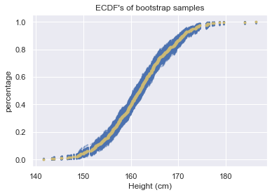
As we can see above, we got different heights, but we can easily detect that the points are spreading in a specific range. That’s the confidence interval that we want to learn

正如我们在上面看到的，我们得到了不同的高度，但是我们可以轻松地检测到这些点在特定范围内扩展。 那就是我们要学习的置信区间

You may say that it is impossible to repeat the experiment so many times, you are not wrong. The exact reason why we use the Bootstrap Method. It helps us to simulate the same experiment thousands or even billions of times.

您可能会说不可能重复这么多次实验，您是对的。 我们使用Bootstrap方法的确切原因。 它可以帮助我们模拟同一实验数千甚至数十亿次。

How?

怎么样？

In fact, the Bootstrap Method is quite straightforward and easy to understand. First, it generates bootstrap samples from our original sample by randomly choosing among the original sample. After that, it applies a summary statistics such as variation, standard deviation, mean, and so forth to get replicates. We will use ‘mean’ to generate our bootstrap replicates.

实际上，Bootstrap方法非常简单易懂。 首先，它通过从原始样本中随机选择来从我们的原始样本中生成引导样本。 之后，它应用摘要统计信息(例如变异，标准偏差，均值等)来获得重复数据。 我们将使用“均值”来生成引导程序副本。

To understand the method, let’s apply it to a small sample that contains only 5 heights. We can generate our bootstrap samples like the following. Do not forget the fact that we can choose any observation more than once (resampling with replacement)

为了理解该方法，让我们将其应用于仅包含5个高度的小样本。 我们可以生成如下所示的引导程序示例。 不要忘记我们可以多次选择任何观测值的事实(通过替换进行重采样)

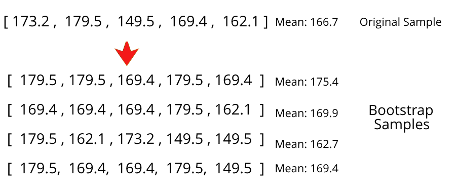
As we can see above we create 4 bootstrap samples and after that calculate their means. We will call these means our bootstrap replicates. Instead of ‘mean’ we could choose variance, standard deviation, median, or anything else.

正如我们在上面看到的，我们创建了4个引导程序样本，然后计算它们的均值。 我们将这些称为“引导复制”。 除了“均值”，我们可以选择方差，标准差，中位数或其他任何值。

Come back to our project. The next step, we are going to generate our bootstrap sample from our original sample and we will apply to mean to get bootstrap replicate. We will repeat this process 15.000 times (drawing) in a for loop and store the replicates in an array. To do this we can define a function like following

回到我们的项目。 下一步，我们将从原始样本中生成引导样本，并将应用于以获得引导复制。 我们将在for循环中重复此过程15.000次(绘制)，并将重复项存储在数组中。 为此，我们可以定义如下函数

After we got 15.000 replicates by calling the function, we can compare between the means of the original sample and the bootstrap replicates

通过调用函数获得15.000个复制后，我们可以在原始样本的均值和引导复制之间进行比较

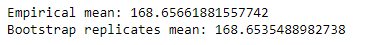
Their means are too close.

他们的手段太接近了。

So, what are we going to do to calculate a 95% confidence interval?

那么，我们要怎么做才能计算出95％的置信区间？

After obtaining bootstrap replicates, the rest is so simple. As we know, our lower and upper limits are the values correspond to the 2.5th and 97.5th percentiles.

获得引导程序副本后，其余的操作非常简单。 众所周知，我们的下限和上限分别是2.5％和97.5％的值。

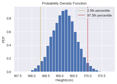
We can find the boundaries with following simple Python code

我们可以通过以下简单的Python代码找到边界

Our boundaries are found at 167.7 and 169.5. Therefore, we can say that if we do the same experiment with the whole population. The mean of heights will be between 167.7 cm and 169.5 cm with 95% of chance

我们的边界位于167.7和169.5。 因此，可以说，如果对整个人口进行相同的实验。 身高的平均值在167.7厘米至169.5厘米之间，有95％的机会

摘要 (Summary)

Let’s summarize what we did. We have randomly selected 500 heights and generated bootstrap samples. We calculated the ‘mean’ from those samples and got bootstrap replicates of means. Ultimately we calculated a 95% confidence interval.

让我们总结一下我们所做的。 我们随机选择了500个高度并生成了引导程序样本。 我们从这些样本中计算出“均值”，并获得了均值的自举重复项。 最终，我们计算出95％的置信区间。

I wish you good luck in your data journey :)

祝您在数据旅途中一切顺利：)